california-real-estate

California Housing Prices

California Housing dataset suggests the median housing prices for the year 1990 during which the U.S Census Bureau was responsible for housing data. In this report, we discover how well our model manages when the same data can be used to predict today’s median price for each block group. In doing so, the model can differentiate between different blocks, provide essential information to buyers and predict concurrent datasets given the independent variables.

We will try to answer the following questions with context to our topic:
What is the inflation rate from 1990 to 2021?
Can we determine median housing price based on independent factors?
Is the change in California Housing prices following linear relationship?
Can we alter the data to reflect inflation costs since 1990?

Data Description

California Housing Dataset has 20640 instances, 8 predictive attributes and the target predictor of numeric data type.

As observed in the following dataset abbreviations, these are the terminologies:

• MedInc: median income in block
• HouseAge: median house age in block
• AveRooms: average number of rooms
• AveBedrms: average number of bedrooms
• Population: block population
• AveOccup: average house occupancy
• Latitude: house block latitude
• Longitude: house block longitude

This dataset was derived from the 1990 U.S. census, using one row per census block group. A block group is the smallest geographical unit for which the U.S. Census Bureau publishes sample data (a block group typically has a population of 600 to 3,000 people).

We see that median house prices and median incomes are having positive linear relationship

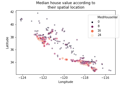
With the help of scatterplot we can see that housing prices are related to the latitude and logitude (location) of the property. Here the color represents the price of the house

# dataset for features and pricing
dataset = pd.DataFrame(df.data,columns=df.feature_names)
dataset["MedHouseVal"] = df.target

No missing values were found in this dataset. The target variable is the median house value for California districts.

Adjusting for inflation in 2021.

# multiplying target values by 4.4
dataset["MedHouseVal"] = dataset["MedHouseVal"] * 4.4

We check for outlier data using the boxplot() by seaborn. The outlier data is the one that lies outside the lower & upper limits.

# checking for outliers
for i in dataset.columns:
    plt.figure(figsize=(4,5))
    plt.title(i)
    plt.boxplot(dataset[i])
    plt.show()

checking for outliers

outliers = dataset[(dataset["MedInc"]>8)&(dataset["AveRooms"]>9)&(dataset["AveBedrms"]>1.25)&(dataset["MedHouseVal"]>21)]

After dropping 5 records, dataset has 20635 instances

Proposed Model and Justification

We use StandardScaler, MinMaxScaler and RobustScaler, the scaling technique that produces the best score is used further.
Implement Principal Component Analysis (PCA) on the scaled features to reduce dimensionality of data and prevent low scorers from feature selection.
Implement Polynomial Features as an alternative to PCA which will be defined in the second scenario.
Once the features are scaled and filtered, records separated into training and testing subsets of dataset with each having their own independent and dependent variables.
After splitting the dataset into training and testing sets, apply the following regression techniques: Linear Regression, Lasso Regression, Ridge Regression, Decision Tree Regression, Random Forest Regression, Gradient Boost Regressor, MLP Regression.

Modelling aims has the following objectives:

• Data we possess is not relevant and therefore must scale the dependent variable to reflect inflation.
• Model should reduce dimensionality of data, prevent low scorers from feature selection, polishing record classifications with outlier data and pipelining multiple functions to reduce CPU time
• Our regression model should evaluate multiple parameters in pursuit of best r2, RMSE and mean accuracy score.
• Datasets must be split into training and testing subsets of data with each having their own independent and dependent variables. Meanwhile, out of sample data taken from training set as validation set marks the overall scores.

Results

Plots and Summary Tables We see the results for the cumulative sum of variances of scaled features with respect to number of dimensions.

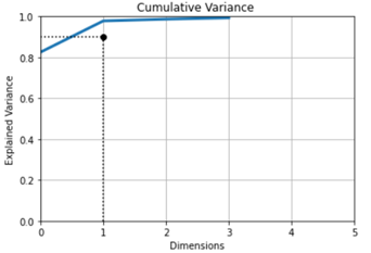
From the Explained Variance Ratio, we see that

• 1st variable explains 0.83%
• 2nd variable explains 0.15%
• 3rd variable 0.01%
• 4th variable 0.01% of the total variance
• which means that 0.01 is lost.

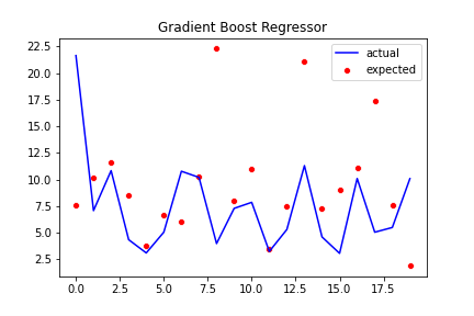
Best model we obtain from Prediction with PCA:

• Best model Training R2 score: 57.85%
• Best model Testing R2 score: 54.04%
• Best RMSE score: 3.42
• Best Average CV score: 55%

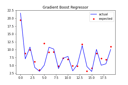
Best model we obtain from Prediction with Polynomial Features:

• Best model Training R2 score: 80.84%
• Best model Testing R2 score: 78.42%
• Best RMSE score: 2.34
• Best Average CV score: 78%

Assessment

• The model appears valid and uses the common parameters to fit the target variable accurately. It then performs the testing predictions with good accuracy.
• Although training r2 score is quite large for the models, testing r2 score is more valuable as it represents the dataset not fitted on.
• Root mean square error defines the square root of the sum of squaring the difference between the actual and predicted values.
• α parameter values define the regularization term weight associated with the model. Defining multiple parameter values increases chance of best mean accuracy score.
• The best model can predict data for our testing set with a mean accuracy score of 65%
• We can achieve a better score with Polynomial Features than PCA, therefore, the target variable could be defined into a polynomial function with predictive variables to a degree of 2.

Final model prediction on Out-of-Sample dataset

Our model can predict data for out-of-sample dataset with a mean accuracy score of 79%.

Training R2 score: 80.84% Validation R2 score: 78.10% Validation RMSE score 2.37 Average CV score: 79%

From the results shown, we will conclude saying our model can predict results with 79% accuracy and is prone to underfitting.

Concluding Remarks

• Prediction: We can predict with adequate accuracy the median housing prices for year 2021
• Outlier data: The dataset contains more outliers that caused the predictions to drop when removed
• Insufficient data: More records are necessary achieve higher mean accuracy and reduce variance
• Inconsistent data: Dataset published in 1990 has been adjusted to reflect some inflation